Analysis of Starbucks Beverages
Contribution to TidyTuesday, week 52
This year-end was quite busy, between organizing the VI Meeting of Researchers in Development, Learning and Education and writing two! papers. And without even considering the pandemic.
I had been wanting to do something for #TidyTuesday, but the latest proposals didn’t motivate me much. Don’t get me wrong, I love the Spice Girls and spiders are nice (although I couldn’t say I’m very interested in cricket), but the types of data they brought weren’t particularly engaging for me. While this project aims to work on visualization tools, what I need most right now is to improve my statistical skills.
That’s why I chose this week: data on Starbucks beverages. The dataset has a lot of numerical information that will allow me to reproduce a basic statistical analysis. Let’s start by importing and organizing the data a bit.
tuesdata <- tidytuesdayR::tt_load('2021-12-21')## ---- Compiling #TidyTuesday Information for 2021-12-21 ----
## --- There is 1 file available ---
##
##
## ── Downloading files ───────────────────────────────────────────────────────────
##
## 1 of 1: "starbucks.csv"starbucks <- tuesdata$starbucks
starbucks$product_name <- as.factor(starbucks$product_name)
starbucks$size <- as.factor(starbucks$size)
starbucks$milk <- as.factor(starbucks$milk)
starbucks$whip <- as.factor(starbucks$whip)
starbucks$trans_fat_g <- as.numeric(starbucks$trans_fat_g)
starbucks$fiber_g <- as.numeric(starbucks$fiber_g)Descriptive Analysis
To understand a bit more about how these beverages are composed, we will perform a descriptive analysis. We have two size measures (size and serve_size_m_l), calories, total fats (saturated fats and trans fats), grams of cholesterol, grams of sodium, total carbohydrates, grams of fiber, grams of sugar, and grams of caffeine.
The first thing we’re going to do is see how the beverages are distributed according to the quantity of these ingredients. However, I encountered the problem that the different elements appear, even within their distribution, with very different absolute values. This makes them not clearly distinguishable if I present them all in the same graph. I will therefore maintain the separation by sizes, but I will only work with standard sizes (short, tall, venti, grande).
library(tidyverse)## Warning: package 'tibble' was built under R version 4.4.1## Warning: package 'purrr' was built under R version 4.4.1## Warning: package 'stringr' was built under R version 4.4.1## ── Attaching core tidyverse packages ──────────────────────── tidyverse 2.0.0 ──
## ✔ dplyr 1.1.4 ✔ readr 2.1.5
## ✔ forcats 1.0.0 ✔ stringr 1.6.0
## ✔ ggplot2 3.5.1 ✔ tibble 3.3.0
## ✔ lubridate 1.9.3 ✔ tidyr 1.3.1
## ✔ purrr 1.2.0
## ── Conflicts ────────────────────────────────────────── tidyverse_conflicts() ──
## ✖ dplyr::filter() masks stats::filter()
## ✖ dplyr::lag() masks stats::lag()
## ℹ Use the conflicted package (<http://conflicted.r-lib.org/>) to force all conflicts to become errorsstarbucks_longer <- starbucks %>%
mutate(caffeine_g = caffeine_mg*100,
cholesterol_g = cholesterol_mg*100,
sodium_g = sodium_mg*100) %>%
select(-c(caffeine_mg, cholesterol_mg, sodium_mg)) %>%
pivot_longer(cols = c(5:15),
names_to = "character",
values_to = "n")
starbucks_longer$size <- factor(starbucks_longer$size, levels = c("short", "tall", "grande", "venti"))
starbucks_longer %>%
filter(character %in% c("calories", "total_fat_g", "sodium_g", "cholesterol_g", "fiber_g", "sugar_g", "caffeine_g")) %>%
filter(size %in% c("short", "tall", "venti", "grande")) %>%
ggplot()+
geom_density(mapping = aes(n, color = size))+
facet_wrap(~character, scales = "free")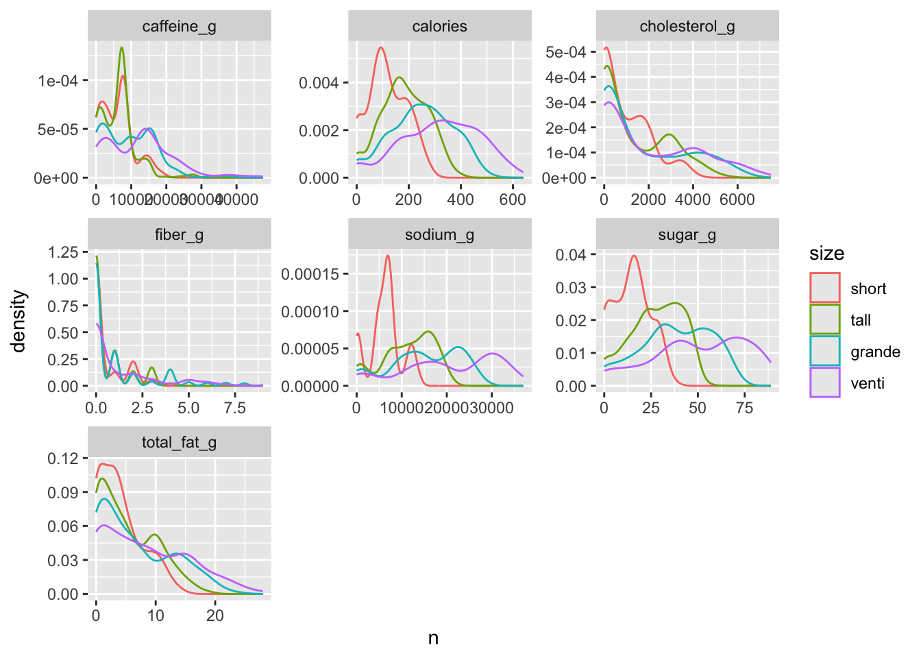
In principle, it can be seen that, broadly speaking, the graphs follow a logical pattern: larger sizes have flatter distributions, while smaller sizes have more pronounced peaks. The caffeine graph particularly catches my attention: both “short” and “tall” sizes have very similar peaks (a lot of caffeine for a small size or little caffeine for a larger size?). It is possible, however, that not all types of beverages come in all four sizes, and that this introduces biases into the graphs. We will see this later.
starbucks_longer %>%
  filter(character %in% c("calories", "total_fat_g", "sodium_g", "cholesterol_g", "fiber_g", "sugar_g", "caffeine_g")) %>%
  filter(size %in% c("short", "tall", "venti", "grande")) %>%
  ggplot()+
  geom_boxplot(mapping = aes(x = size, y = n, fill = size))+
  facet_wrap(~character, scales = "free")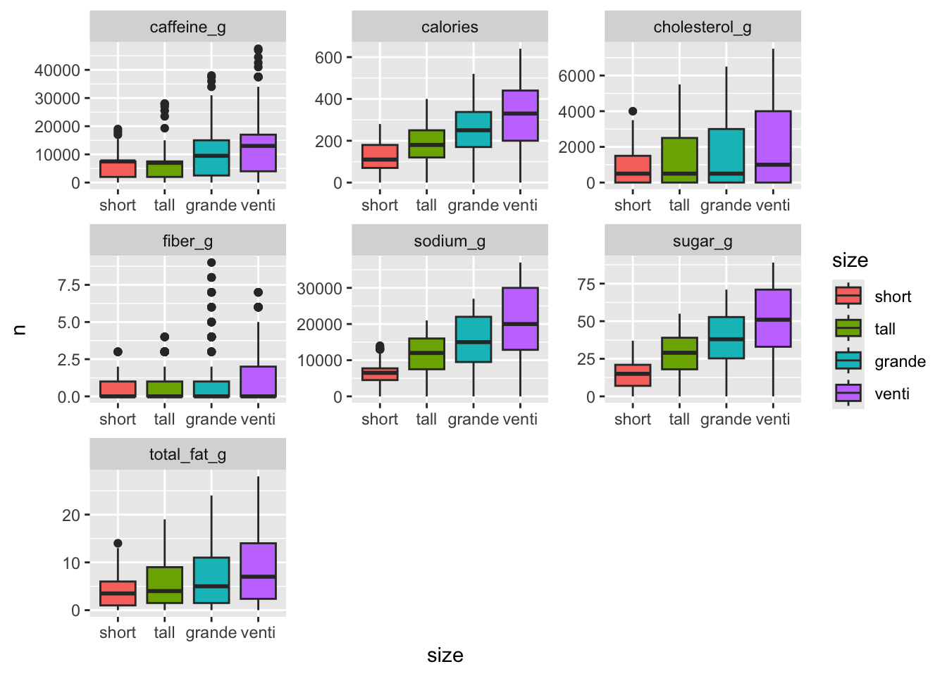
The boxplot more clearly shows the difference between sizes, which nonetheless continues to show similarities in the first two sizes for both caffeine and fiber content. A good question for later is: are there statistically significant differences between the amount of caffeine in beverages of the first two sizes?
Now, which beverages have the highest amount of each element? To compare, we will stick to the smallest versions (“short”), without considering other characteristics:
library(gt)## Warning: package 'gt' was built under R version 4.4.1library(gtExtras)
starbucks %>%
filter(size == "short") %>%
arrange(desc(caffeine_mg)) %>%
select(product_name, caffeine_mg) %>%
unique() %>%
slice_head(n =10) %>%
gt() %>%
tab_options(
column_labels.text_transform = "Product Name"
) %>%
tab_header(title = "Top 10 Products with the Most Caffeine") %>%
gt_theme_nytimes() %>%
tab_source_note(source_note = "Source: Starbucks Coffee Company | Made by @_msquiroga for #TidyTuesday") %>%
cols_align("left")| Top 10 Products with the Most Caffeine | |
| product_name | caffeine_mg |
|---|---|
| Clover Brewed Coffee - Dark Roast | 190 |
| brewed coffee - True North Blend Blonde roast | 180 |
| Clover Brewed Coffee - Medium Roast | 170 |
| brewed coffee - medium roast | 155 |
| Clover Brewed Coffee - Light Roast | 155 |
| Latte Macchiato | 150 |
| brewed coffee - dark roast | 130 |
| Flat White | 130 |
| Caffè Mocha | 90 |
| Caffè Misto | 75 |
| Source: Starbucks Coffee Company | Made by @_msquiroga for #TidyTuesday | |
So, friends: if you need a little help to start your day, you can stop by your nearest Starbucks and order a Clover Brewed Coffee - Dark Roast (if it exists in your countries, of course: I don’t think it does in mine).
Regression
I started this post by stating that I wanted to practice my statistical skills, but I’m no longer so sure that this dataset will give me many opportunities for major operations. For now, I’ll stick with this question: what aspect of beverage composition contributes significantly most to the total fat content? Of course, this is an answer that can be obtained from a nutritional point of view: the presence of milk and cream, along with the size of the beverage, should be the three most significant predictors. But let’s see if statistics supports us.
starbucks <- starbucks %>%
  filter(!size %in% c("1 scoop", "1 shot"))

fat_reg <- lm(total_fat_g ~ size + milk + whip + serv_size_m_l + calories + cholesterol_mg + sodium_mg + fiber_g + sugar_g + caffeine_mg, data  = starbucks)
summary(fat_reg)
##
## Call:
## lm(formula = total_fat_g ~ size + milk + whip + serv_size_m_l +
## calories + cholesterol_mg + sodium_mg + fiber_g + sugar_g +
## caffeine_mg, data = starbucks)
##
## Residuals:
## Min 1Q Median 3Q Max
## -4.5403 -0.5246 0.0487 0.5103 7.6863
##
## Coefficients:
## Estimate Std. Error t value Pr(>|t|)
## (Intercept) -0.2538835 0.4009213 -0.633 0.5267
## sizegrande -1.2414507 0.6557588 -1.893 0.0586 .
## sizequad -0.7248447 0.5507526 -1.316 0.1884
## sizeshort -0.2524751 0.4828904 -0.523 0.6012
## sizesolo 0.4126085 0.5473979 0.754 0.4511
## sizetall -0.5817991 0.5569494 -1.045 0.2964
## sizetrenta -1.5889205 1.0794471 -1.472 0.1413
## sizetriple -0.3613976 0.5473937 -0.660 0.5093
## sizeventi -1.8653208 0.8295612 -2.249 0.0247 *
## milk1 -2.5098877 0.1339820 -18.733 < 2e-16 ***
## milk2 -1.5945736 0.1510997 -10.553 < 2e-16 ***
## milk3 -0.9801896 0.1475690 -6.642 4.81e-11 ***
## milk4 0.9084118 0.1445475 6.285 4.70e-10 ***
## milk5 -0.6896911 0.1582705 -4.358 1.43e-05 ***
## whip1 1.8390692 0.1669839 11.013 < 2e-16 ***
## serv_size_m_l 0.0021254 0.0011338 1.875 0.0611 .
## calories 0.0688260 0.0013809 49.842 < 2e-16 ***
## cholesterol_mg 0.0416803 0.0064425 6.470 1.46e-10 ***
## sodium_mg 0.0047823 0.0007800 6.131 1.20e-09 ***
## fiber_g -0.5514295 0.0284809 -19.361 < 2e-16 ***
## sugar_g -0.2720957 0.0062719 -43.383 < 2e-16 ***
## caffeine_mg -0.0003979 0.0004756 -0.837 0.4029
## ---
## Signif. codes: 0 '***' 0.001 '**' 0.01 '*' 0.05 '.' 0.1 ' ' 1
##
## Residual standard error: 1.022 on 1122 degrees of freedom
## Multiple R-squared: 0.9712, Adjusted R-squared: 0.9707
## F-statistic: 1801 on 21 and 1122 DF, p-value: < 2.2e-16The first thing I always look at is that the model is significant: we can see this with the p-value that appears at the end of the summary. Indeed, the model appears to be significant; in other words, the description of the situation we proposed is supported by the data. Furthermore, the $R^2$ is very high.
Now, let’s look at the variables. Size only turned out to be a significant predictor for the largest size, “venti”. This strongly catches my attention, because I had predicted that as size increased, the total fat content would also increase, but it’s possible that when controlling for other variables, size no longer plays an important role (perhaps because the beverage composition changes? because everything always has a lot of fat?).
The presence of milk and cream was, as I had predicted, a significant predictor in all cases. This is, of course, logical from a nutritional point of view. The same applies to the calorie count: as far as I understand, calories are a measure of energy produced by fats, proteins, and carbohydrates. Therefore, while it is logical that it turned out to be a significant predictor, it should not have appeared in the model from the perspective of the underlying theory. Cholesterol was also a significant predictor, which is logical because it is a type of fat.
What strikes me is that sodium, fiber, and sugar were also statistically significant predictors. Again, my basic nutritional knowledge tells me that these elements should not contribute to total fat content, but it’s possible that the ingredients that provide these elements also contain high levels of fats. It is therefore crucial to thoroughly understand the elements we work with when proposing a statistical model.
Finally, we can analyze the model’s residuals to get a clearer picture.
library(performance)## Warning: package 'performance' was built under R version 4.4.1performance::check_model(fat_reg)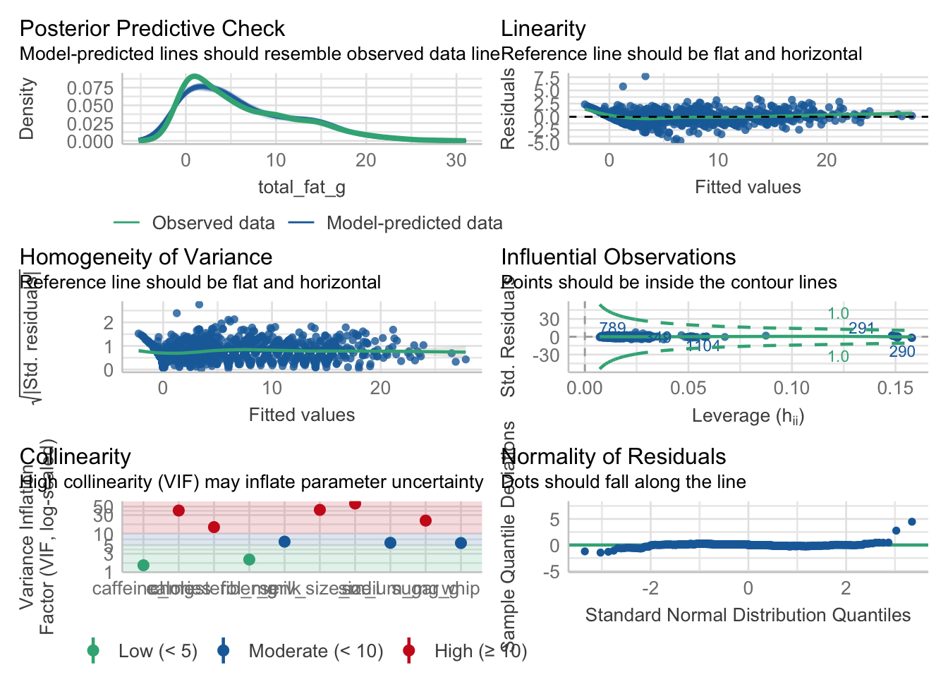
The residual analysis shows several of the things mentioned earlier: for example, the high degree of collinearity among several ingredients. Linearity and homogeneity of variance clearly have very strange shapes, and I wonder if it has to do with the different sizes, which propose different ingredient compositions from the same formulas. I believe a more appropriate methodology would be to run different models for each size, to be able to compare between beverages (i.e., between recipes).
In short, the residual analysis shows, as we already knew, that although the model summary initially yielded seemingly significant results, the residual analysis reveals that there are some issues that are overlooked and that this model would not be the most appropriate for this scenario. This analysis could be continued, as I mentioned before, by running different models for each size, proposing correlations between ingredients to detect problematic collinearities. But this was enough for today. Thanks for reading!
Macarena Quiroga
Linguist/PhD student
I research language acquisition. I’m looking to deepen my knowledge of statistis and data science with R/Rstudio. If you like what I do, you can buy me a coffee from Argentina, or a kofi from other countries. Suscribe to my blog here.