Choroplethr maps about USA drought with R
The theme for week 24 of #TidyTuesday is drought in the US and when I read about the amount of precipitation per year I immediately thought it was a great opportunity to play with raincloud plots. However, the data was not on my side, because it presented temporal-spatial information. So I decided to continue with my approach to spatial data management.
Luckily a few months ago I had signed up for Ari Lamstein’s Choropleth Maps course, so I had material from where to start.
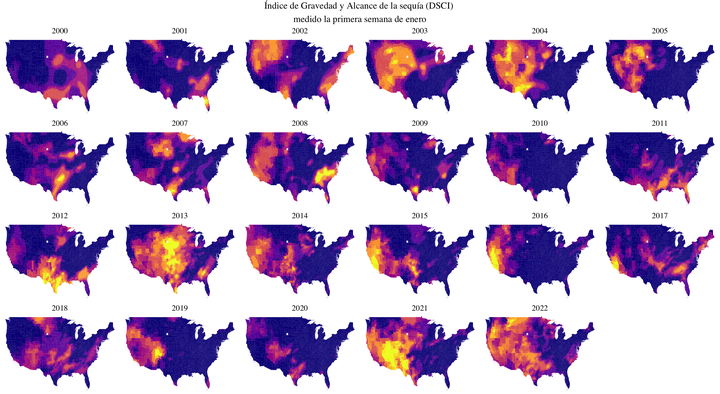
One of the TidyTuesday datasets has the Drought Severity and Coverage Index (DSCI) along with the FIPS code indicating the county and state. This FIPS code is the same one that appears with the region name in the map from the choroplethrMaps package.
So, I load the necessary packages and the map of the counties:
tuesdata <- tidytuesdayR::tt_load('2022-06-14')##
## Downloading file 1 of 2: `drought.csv`
## Downloading file 2 of 2: `drought-fips.csv`drought <- tuesdata$drought
drought_fips <- tuesdata$`drought-fips`
library(choroplethr)
library(choroplethrMaps)
library(tidyverse)
data("county.map")Now I can rename the corresponding values in the drought dataframe so that I can use it as the basis for the choropleth map. I also need to specify that the DSCI value (now called “value”) be numeric, not character. With this, I am now able to merge the counties geodata df (county.map) with my drought data df (drought.fips):
drought_fips <- drought_fips %>%
  rename(region = FIPS,
         value = DSCI)

drought_fips$region <- as.numeric(drought_fips$region)

county.map.drought <- county.map %>%
  left_join(drought_fips, by = "region") %>%
select(long, lat, region, value, date, STATE, group)## Warning in left_join(., drought_fips, by = "region"): Detected an unexpected many-to-many relationship between `x` and `y`.
## ℹ Row 1 of `x` matches multiple rows in `y`.
## ℹ Row 35131 of `y` matches multiple rows in `x`.
## ℹ If a many-to-many relationship is expected, set `relationship =
## "many-to-many"` to silence this warning.It only remains to generate the graphs for each year one by one: I select the date of the first measurement of the year and eliminate the states of Alaska and the Hawaiian Islands (only because it makes mapping difficult, it is nothing personal):
# 2000
a2000 <- county.map.drought %>%
  filter(date == "2000-01-04" & !STATE %in% c("02", "15")) %>%
  ggplot(aes(long, lat, group=group)) +
  geom_polygon(aes(fill = value))+
  scale_fill_viridis_c(option = "plasma",
                       limits = c(0, 500))+
  labs(title = "2000",
       x = "", y = "")+
  theme_void()+
  theme(legend.position = "none",
        plot.title = element_text(size = 12, hjust = 0.5,
                                  family="Times"))

# 2001
a2001 <- county.map.drought %>%
  filter(date == "2001-01-02" & !STATE %in% c("02", "15")) %>%
  ggplot(aes(long, lat, group=group)) +
  geom_polygon(aes(fill = value))+
  scale_fill_viridis_c(option = "plasma",
                       limits = c(0, 500))+
  labs(title = "2001",
       x = "", y = "")+
  theme_void()+
  theme(legend.position = "none",
        plot.title = element_text(size = 12, hjust = 0.5,
                                  family="Times"))

# 2002
a2002 <- county.map.drought %>%
  filter(date == "2002-01-01" & !STATE %in% c("02", "15")) %>%
  ggplot(aes(long, lat, group=group)) +
  geom_polygon(aes(fill = value))+
  scale_fill_viridis_c(option = "plasma",
                       limits = c(0, 500))+
  labs(title = "2002",
       x = "", y = "")+
  theme_void()+
  theme(legend.position = "none",
        plot.title = element_text(size = 12, hjust = 0.5,
                                  family="Times"))

# 2003
a2003 <- county.map.drought %>%
  filter(date == "2003-01-07" & !STATE %in% c("02", "15")) %>%
  ggplot(aes(long, lat, group=group)) +
  geom_polygon(aes(fill = value))+
  scale_fill_viridis_c(option = "plasma",
                       limits = c(0, 500))+
  labs(title = "2003",
       x = "", y = "")+
  theme_void()+
  theme(legend.position = "none",
        plot.title = element_text(size = 12, hjust = 0.5,
                                  family="Times"))

# 2004
a2004 <- county.map.drought %>%
  filter(date == "2004-01-06" & !STATE %in% c("02", "15")) %>%
  ggplot(aes(long, lat, group=group)) +
  geom_polygon(aes(fill = value))+
  scale_fill_viridis_c(option = "plasma",
                       limits = c(0, 500))+
  labs(title = "2004",
       x = "", y = "")+
  theme_void()+
  theme(legend.position = "none",
        plot.title = element_text(size = 12, hjust = 0.5,
                                  family="Times"))

# 2005
a2005 <- county.map.drought %>%
  filter(date == "2005-01-04" & !STATE %in% c("02", "15")) %>%
  ggplot(aes(long, lat, group=group)) +
  geom_polygon(aes(fill = value))+
  scale_fill_viridis_c(option = "plasma",
                       limits = c(0, 500))+
  labs(title = "2005",
       x = "", y = "")+
  theme_void()+
  theme(legend.position = "none",
        plot.title = element_text(size = 12, hjust = 0.5,
                                  family="Times"))

# 2006
a2006 <- county.map.drought %>%
  filter(date == "2006-01-03" & !STATE %in% c("02", "15")) %>%
  ggplot(aes(long, lat, group=group)) +
  geom_polygon(aes(fill = value))+
  scale_fill_viridis_c(option = "plasma",
                       limits = c(0, 500))+
  labs(title = "2006",
       x = "", y = "")+
  theme_void()+
  theme(legend.position = "none",
        plot.title = element_text(size = 12, hjust = 0.5,
                                  family="Times"))

# 2007
a2007 <- county.map.drought %>%
  filter(date == "2007-01-02" & !STATE %in% c("02", "15")) %>%
  ggplot(aes(long, lat, group=group)) +
  geom_polygon(aes(fill = value))+
  scale_fill_viridis_c(option = "plasma",
                       limits = c(0, 500))+
  labs(title = "2007",
       x = "", y = "")+
  theme_void()+
  theme(legend.position = "none",
        plot.title = element_text(size = 12, hjust = 0.5,
                                  family="Times"))

# 2008
a2008 <- county.map.drought %>%
  filter(date == "2008-01-01" & !STATE %in% c("02", "15")) %>%
  ggplot(aes(long, lat, group=group)) +
  geom_polygon(aes(fill = value))+
  scale_fill_viridis_c(option = "plasma",
                       limits = c(0, 500))+
  labs(title = "2008",
       x = "", y = "")+
  theme_void()+
  theme(legend.position = "none",
        plot.title = element_text(size = 12, hjust = 0.5,
                                  family="Times"))

# 2009
a2009 <- county.map.drought %>%
  filter(date == "2009-01-06" & !STATE %in% c("02", "15")) %>%
  ggplot(aes(long, lat, group=group)) +
  geom_polygon(aes(fill = value))+
  scale_fill_viridis_c(option = "plasma",
                       limits = c(0, 500))+
  labs(title = "2009",
       x = "", y = "")+
  theme_void()+
  theme(legend.position = "none",
        plot.title = element_text(size = 12, hjust = 0.5,
                                  family="Times"))

# 2010
a2010 <- county.map.drought %>%
  filter(date == "2010-01-05" & !STATE %in% c("02", "15")) %>%
  ggplot(aes(long, lat, group=group)) +
  geom_polygon(aes(fill = value))+
  scale_fill_viridis_c(option = "plasma",
                       limits = c(0, 500))+
  labs(title = "2010",
       x = "", y = "")+
  theme_void()+
  theme(legend.position = "none",
        plot.title = element_text(size = 12, hjust = 0.5,
                                  family="Times"))

# 2011
a2011 <- county.map.drought %>%
  filter(date == "2011-01-04" & !STATE %in% c("02", "15")) %>%
  ggplot(aes(long, lat, group=group)) +
  geom_polygon(aes(fill = value))+
  scale_fill_viridis_c(option = "plasma",
                       limits = c(0, 500))+
  labs(title = "2011",
       x = "", y = "")+
  theme_void()+
  theme(legend.position = "none",
        plot.title = element_text(size = 12, hjust = 0.5,
                                  family="Times"))

# 2012
a2012 <- county.map.drought %>%
  filter(date == "2012-01-03" & !STATE %in% c("02", "15")) %>%
  ggplot(aes(long, lat, group=group)) +
  geom_polygon(aes(fill = value))+
  scale_fill_viridis_c(option = "plasma",
                       limits = c(0, 500))+
  labs(title = "2012",
       x = "", y = "")+
  theme_void()+
  theme(legend.position = "none",
        plot.title = element_text(size = 12, hjust = 0.5,
                                  family="Times"))

# 2013
a2013 <- county.map.drought %>%
  filter(date == "2013-01-01" & !STATE %in% c("02", "15")) %>%
  ggplot(aes(long, lat, group=group)) +
  geom_polygon(aes(fill = value))+
  scale_fill_viridis_c(option = "plasma",
                       limits = c(0, 500))+
  labs(title = "2013",
       x = "", y = "")+
  theme_void()+
  theme(legend.position = "none",
        plot.title = element_text(size = 12, hjust = 0.5,
                                  family="Times"))

# 2014
a2014 <- county.map.drought %>%
  filter(date == "2014-01-07" & !STATE %in% c("02", "15")) %>%
  ggplot(aes(long, lat, group=group)) +
  geom_polygon(aes(fill = value))+
  scale_fill_viridis_c(option = "plasma",
                       limits = c(0, 500))+
  labs(title = "2014",
       x = "", y = "")+
  theme_void()+
  theme(legend.position = "none",
        plot.title = element_text(size = 12, hjust = 0.5,
                                  family="Times"))

# 2015
a2015 <- county.map.drought %>%
  filter(date == "2015-01-06" & !STATE %in% c("02", "15")) %>%
  ggplot(aes(long, lat, group=group)) +
  geom_polygon(aes(fill = value))+
  scale_fill_viridis_c(option = "plasma",
                       limits = c(0, 500))+
  labs(title = "2015",
       x = "", y = "")+
  theme_void()+
  theme(legend.position = "none",
        plot.title = element_text(size = 12, hjust = 0.5,
                                  family="Times"))

# 2016
a2016 <- county.map.drought %>%
  filter(date == "2016-01-05" & !STATE %in% c("02", "15")) %>%
  ggplot(aes(long, lat, group=group)) +
  geom_polygon(aes(fill = value))+
  scale_fill_viridis_c(option = "plasma",
                       limits = c(0, 500))+
  labs(title = "2016",
       x = "", y = "")+
  theme_void()+
  theme(legend.position = "none",
        plot.title = element_text(size = 12, hjust = 0.5,
                                  family="Times"))

# 2017
a2017 <- county.map.drought %>%
  filter(date == "2017-01-03" & !STATE %in% c("02", "15")) %>%
  ggplot(aes(long, lat, group=group)) +
  geom_polygon(aes(fill = value))+
  scale_fill_viridis_c(option = "plasma",
                       limits = c(0, 500))+
  labs(title = "2017",
       x = "", y = "")+
  theme_void()+
  theme(legend.position = "none",
        plot.title = element_text(size = 12, hjust = 0.5,
                                  family="Times"))

# 2018
a2018 <- county.map.drought %>%
  filter(date == "2018-01-02" & !STATE %in% c("02", "15")) %>%
  ggplot(aes(long, lat, group=group)) +
  geom_polygon(aes(fill = value))+
  scale_fill_viridis_c(option = "plasma",
                       limits = c(0, 500))+
  labs(title = "2018",
       x = "", y = "")+
  theme_void()+
  theme(legend.position = "none",
        plot.title = element_text(size = 12, hjust = 0.5,
                                  family="Times"))

# 2019
a2019 <- county.map.drought %>%
  filter(date == "2019-01-01" & !STATE %in% c("02", "15")) %>%
  ggplot(aes(long, lat, group=group)) +
  geom_polygon(aes(fill = value))+
  scale_fill_viridis_c(option = "plasma",
                       limits = c(0, 500))+
  labs(title = "2019",
       x = "", y = "")+
  theme_void()+
  theme(legend.position = "none",
        plot.title = element_text(size = 12, hjust = 0.5,
                                  family="Times"))

# 2020
a2020 <- county.map.drought %>%
  filter(date == "2020-01-07" & !STATE %in% c("02", "15")) %>%
  ggplot(aes(long, lat, group=group)) +
  geom_polygon(aes(fill = value))+
  scale_fill_viridis_c(option = "plasma",
                       limits = c(0, 500))+
  labs(title = "2020",
       x = "", y = "")+
  theme_void()+
  theme(legend.position = "none",
        plot.title = element_text(size = 12, hjust = 0.5,
                                  family="Times"))

# 2021
a2021 <- county.map.drought %>%
  filter(date == "2021-01-05" & !STATE %in% c("02", "15")) %>%
  ggplot(aes(long, lat, group=group)) +
  geom_polygon(aes(fill = value))+
  scale_fill_viridis_c(option = "plasma",
                       limits = c(0, 500))+
  labs(title = "2021",
       x = "", y = "")+
  theme_void()+
  theme(legend.position = "none",
        plot.title = element_text(size = 12, hjust = 0.5,
                                  family="Times"))

# 2022
a2022 <- county.map.drought %>%
  filter(date == "2022-01-04" & !STATE %in% c("02", "15")) %>%
  ggplot(aes(long, lat, group=group)) +
  geom_polygon(aes(fill = value))+
  scale_fill_viridis_c(option = "plasma",
                       limits = c(0, 500))+
  labs(title = "2022",
       x = "", y = "")+
  theme_void()+
  theme(legend.position = "none",
        plot.title = element_text(size = 12, hjust = 0.5,
                                  family="Times"))
Finally, I combine them into a single graph:
library(grid)
library(gridExtra)##
## Attaching package: 'gridExtra'## The following object is masked from 'package:dplyr':
##
## combine## The following object is masked from 'package:acs':
##
## combinegrid.arrange(grobs = list(a2000, a2001, a2002, a2003, a2004, a2005, a2006, a2007, a2008, a2009, a2010,
a2011, a2012, a2013, a2014, a2015, a2016, a2017, a2018, a2019, a2020,
a2021, a2022),
top = grid::textGrob("Índice de Gravedad y Alcance de la sequía (DSCI) \nmedido la primera semana de enero",
gp = gpar(fontsize = 14, fontfamily = "Times")),
nrow = 4)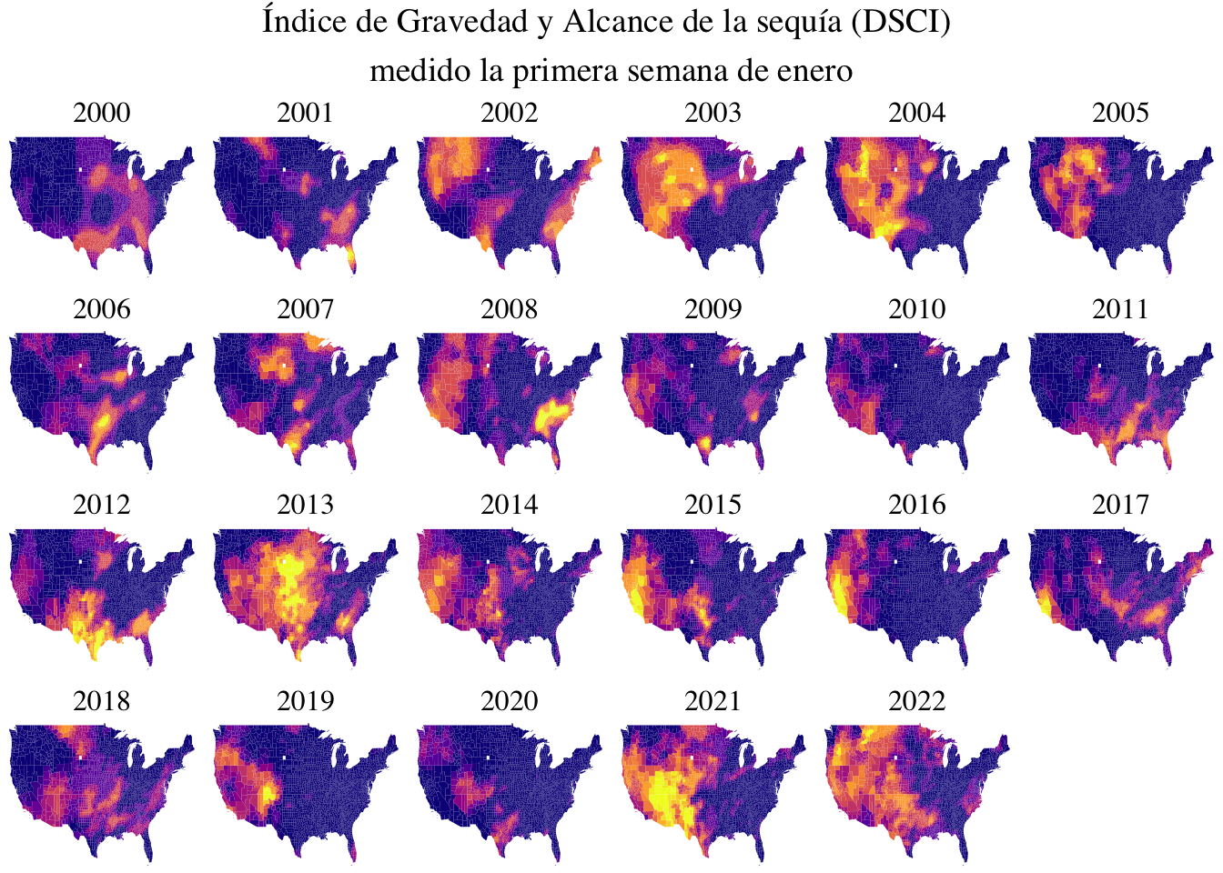
I’m not so sure about the size ratio between the general title and the specific titles for each chart, but for now I’m happy with how it looks.
Now, it’s been great, but is this graph informative? I decided to keep the first week of January for arbitrary reasons, because I was interested in focusing on space. However, it would have been interesting, for example, to make an average per month over the years (that is, to have a map per month that averaged the 22 years of the sample), because it is evident that most of the differences in the levels of drought are going to be seen throughout the year (between seasons, let’s say) than throughout the years. But that implied a handling of the data of dates that I still do not have very clear.
June 2023 update: this blogpost has an updated version where I create a function to reduce lines of code. Check it out!
As always, remember you can suscribe to my blog to stay updated, and if you have any questions, don’t hesitate to contact me. And if you like what I do, you can buy me a cafecito from Argentina or a kofi.
Macarena Quiroga
Linguist/PhD student
I research language acquisition. I’m looking to deepen my knowledge of statistis and data science with R/Rstudio. If you like what I do, you can buy me a coffee from Argentina, or a kofi from other countries. Suscribe to my blog here.