How to Perform a Student's T-Test to Compare Two Groups

Introduction: What is the T-Test?

The Student’s t-test is a statistical technique used to compare the means of two groups and determine if there are significant differences between them. For instance, if we want to know if a specific course in a school had significantly higher grades than another course. In short, very short words (remember, this is not a statistics blog), we can say that the T-test assesses whether the difference between the means of the groups is larger than the within-group variability.

The T-test is a parametric test, which implies that three assumptions must be met: the samples should be independent (meaning that elements from one group do not belong to or influence the elements of the other group), they should follow a normal distribution, and they should be homoscedastic (meaning equal variances). In the case that the samples are heteroscedastic, meaning they have different variances, the Welch statistic can be used for paired samples. If more assumptions are violated, consideration should be given to using non-parametric techniques, such as the Mann-Whitney U test.

Now that we have a rough idea of what the comparison between groups entails, let’s get started!

Step 1: Checking Assumptions

In a previous post, we had begun to analyze the penguins dataset and noticed that male and female penguins had different beak lengths. The question we can ask is: is this difference statistically significant?

We begin by loading the dataset. If you don’t have the palmerpenguins package installed, remove the # symbol from the first line to install it.

install.packages("palmerpenguins")
library(palmerpenguins)
penguins <- penguins

This dataset contains penguins of three different species and from three different islands. Considering the possibility that species may impact beak length and thus complicate the analysis, we will focus solely on the penguins of the first species, Adelie. Later on, we will explore how to analyze the impact of different independent variables (spoiler: using regressions). So, let’s subset the dataset to retain only Adelie penguins:

penguins_adelie <- subset(penguins, species == "Adelie")

The subset function allows us to select a dataset (penguins, the first argument) and extract only those rows that meet the specified condition, in this case, where the species is “Adelie” (note the use of the equivalence operator ==, double equal; you can check the basic operators in this post). We save this subset as a new object named penguins_adelie using the assignment operator <-. It’s essential to verify that this new object appears in the Environment (top-right panel, if you haven’t modified it).

We start by testing the assumption of independent samples: even though the penguins in this sample belong to the same species and coexist on the same island, the assignment of “male” and “female” in this case is not mutually influencing. Therefore, we can assume the independence of samples.

The second assumption is that the distribution is normal. We have two tools for this: the qq plot and the Shapiro-Wilk test. There are various functions available to create a qq plot with different packages. Here, we will use the ggqqplot() function from the ggpubr package.

The code to create a qq plot is as follows: the first line installs the package (this line is commented, but if you haven’t installed the package, remove the # to execute it). The second line loads the package (essential), and the third line executes the code. Within the ggqqplot() function, there are three arguments: the first selects the dataframe we’ll work with, the second selects the variable to plot, and the third selects the grouping variable.

# install.packages("ggpubr)
library(ggpubr)
ggqqplot(penguins_adelie, "bill_length_mm", facet.by = "sex")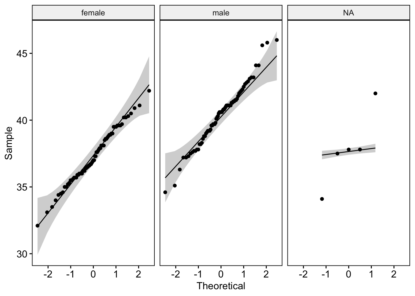

Now it gets a bit tricky. In theory, for the distribution to be normal, the points should all lie on the reference line within the confidence interval (the gray area). If we were purists, we might argue that some points, especially in male penguins, deviate from this interval, suggesting that the sample might not be normal. However, when asked how to interpret the plot, most experts admitted that they often “eyeball” it – meaning they judge it informally. It’s an imprecise answer, I know.

Fortunately, we have another tool to assess normality: the Shapiro-Wilk test.

shapiro.test(penguins_adelie$bill_length_mm[penguins_adelie$sex == "male"])

## 
## 	Shapiro-Wilk normality test
## 
## data:  penguins_adelie$bill_length_mm[penguins_adelie$sex == "male"]
## W = 0.98613, p-value = 0.6067

If we were to translate this line of code into plain language, it would be: apply the Shapiro-Wilk test (shapiro.test()) to the bill_length_mm variable of the penguins_adelie dataframe (penguins_adelie$bill_length_mm) for those rows where the sex is male ([penguins_adelie$sex == "male"]). The $ symbol and the brackets [] are used to subset dataframes.

To interpret the test result, we look at the p-value, which in this case is 0.6067. Since it’s greater than 0.05, we cannot reject the null hypothesis (in this case, the null hypothesis is that the sample has a normal distribution). For the sake of thoroughness, let’s also check the females, although the plot already indicates that their distribution is fairly normal:

shapiro.test(penguins_adelie$bill_length_mm[penguins_adelie$sex == "female"])

## 
## 	Shapiro-Wilk normality test
## 
## data:  penguins_adelie$bill_length_mm[penguins_adelie$sex == "female"]
## W = 0.99117, p-value = 0.8952

So, we have confirmed our second assumption: the samples have a normal distribution. We only need to test the third assumption: homoscedasticity of variances. For this, we use the Levene test, found in the car package:

library(car)

## Loading required package: carData

leveneTest(bill_length_mm ~ sex, data = penguins_adelie)

## Levene's Test for Homogeneity of Variance (center = median)
##        Df F value Pr(>F)
## group   1  0.1744 0.6768
##       144

Within the function, we specify the formula first (bill_length_mm ~ sex), followed by the dataframe to use (data = penguins_adelie). The formula structure will remain the same for all statistical functions involving dependent and independent variables or group comparisons. It’s important to understand this syntax, as it will recur in all such statistical functions. The ~ symbol is called a tilde (find it on your keyboard, or use Alt + 126).

The result of the Levene test does not reject the null hypothesis of equal variances since the p-value is greater than 0.05. Therefore, the assumption of homoscedasticity is met.

Step 2: Student’s T-Test

Now we can effectively move on to using the Student’s T-test. The syntax is quite similar to that of the Levene test, with the only difference being that we specify that the variances are equal (otherwise, the Welch test would be used):

t.test(bill_length_mm ~ sex, data = penguins_adelie, var.equal = T)

## 
## 	Two Sample t-test
## 
## data:  bill_length_mm by sex
## t = -8.7765, df = 144, p-value = 4.44e-15
## alternative hypothesis: true difference in means between group female and group male is not equal to 0
## 95 percent confidence interval:
##  -3.838435 -2.427319
## sample estimates:
## mean in group female   mean in group male 
##             37.25753             40.39041

The p-value is 4.44e-15, in scientific notation. You can disable scientific notation using the following code:

options(scipen = 9999)

Then, re-run the Student’s T-test code: the p-value result will now be 0.00000000000000444. Since this is less than 0.05, we can consider it a significant result, indicating actual differences in beak length between male and female Adelie penguins. To report this in a scholarly article, you can use the following format:

The Student’s T-test revealed statistically significant differences between male and female Adelie penguins (t(144) = -8.77, p < 0.05).

Conclusion

In this post, we explored how to assess the necessary assumptions for running a Student’s T-test for comparing two groups. We also examined the syntax for conducting this test and the method of reporting the results in a scientific article. This test is only applicable for comparing two groups. If you have more than two groups (e.g., to assess whether beak length varies among the three species), you should utilize an ANOVA.

As always, remember you can subscribe to my blog to stay updated, and if you have any questions, feel free to contact me. If you enjoy my work, you can buy me a cup of coffee from Argentina or a kofi from other countries.