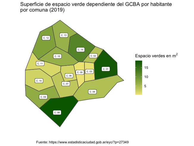
First approach to choropleth map: green spaces in Buenos Aires
Who doesn’t love those beautiful and colorful choropleth maps that circulate on Twitter?
In general, 99% of my use of R is statistical analysis: sometimes I get lucky and can spend a little more time supplementing that analysis with some graphics. But my daily work doesn’t involve with spatial data, so I don’t have much opportunity to learn this kind of stuff.
I had some free time today and first thought I’d do some #TidyTuesday. But looking at the data (bird baths in Australia), I realized that I was geared towards either working with categorical variables or working with spatial data. I had already done some practice with categorical data with Star Trek voice commands, so I ruled that out, but doing something with spatial data seemed a bit complex to me.
I decided then that it was a good opportunity to start step-by-step on that subject and I remembered the existence of PoliticaArgentina, a universe of packages about Argentina. Luckily, the readme had an example of how to make a graph with labels, so it wasn’t hard to adapt it to something new.
I kept the map of CABA (City of Buenos Aires = Ciudad Autónoma de Buenos Aires), because it was what I knew, and I raised a question that matters to any porteño: are there enough green spaces in the City?
Once the graph was assembled, I looked for official information on green spaces in CABA, data that luckily I found on the [official site]((https://www.estadisticaciudad.gob.ar/eyc/?p=27349). Then it was a matter of revising the fill argument and improving the look of the labels a bit. The truth is, I was very satisfied: I thought it would be much more difficult to start, and yet here we are.
Here is the code:
# Choropleth map about green spaces in Buenos Aires

library(tidyverse)
## ── Attaching core tidyverse packages ──────────────────────── tidyverse 2.0.0 ──
## ✔ dplyr 1.1.2 ✔ readr 2.1.4
## ✔ forcats 1.0.0 ✔ stringr 1.5.0
## ✔ ggplot2 3.4.2 ✔ tibble 3.2.1
## ✔ lubridate 1.9.2 ✔ tidyr 1.3.0
## ✔ purrr 1.0.1
## ── Conflicts ────────────────────────────────────────── tidyverse_conflicts() ──
## ✖ dplyr::filter() masks stats::filter()
## ✖ dplyr::lag() masks stats::lag()
## ℹ Use the conflicted package (<http://conflicted.r-lib.org/>) to force all conflicts to become errors#devtools::install_github("politicaargentina/geoAr")
library(geoAr)
show_arg_codes()## # A tibble: 26 × 5
## id codprov codprov_censo codprov_iso name_iso
## <chr> <chr> <chr> <chr> <chr>
## 1 ARGENTINA " " " " AR Argentina
## 2 CABA "01" "02" AR-C Ciudad Autónoma de Buenos Air…
## 3 BUENOS AIRES "02" "06" AR-B Buenos Aires
## 4 CATAMARCA "03" "10" AR-K Catamarca
## 5 CORDOBA "04" "14" AR-X Córdoba
## 6 CORRIENTES "05" "18" AR-W Corrientes
## 7 CHACO "06" "22" AR-H Chaco
## 8 CHUBUT "07" "26" AR-U Chubut
## 9 ENTRE RIOS "08" "30" AR-E Entre Ríos
## 10 FORMOSA "09" "34" AR-P Formosa
## # ℹ 16 more rows(CABA <- get_geo(geo = "CABA"))## Simple feature collection with 15 features and 2 fields
## Geometry type: MULTIPOLYGON
## Dimension: XY
## Bounding box: xmin: -58.52998 ymin: -34.70617 xmax: -58.33444 ymax: -34.53144
## Geodetic CRS: WGS 84
## # A tibble: 15 × 3
## codprov_censo coddepto_censo geometry
## * <chr> <chr> <MULTIPOLYGON [°]>
## 1 02 001 (((-58.34802 -34.601, -58.34713 -34.62111, -58.…
## 2 02 002 (((-58.37501 -34.57959, -58.39365 -34.60154, -5…
## 3 02 003 (((-58.39189 -34.62916, -58.4125 -34.63227, -58…
## 4 02 004 (((-58.33444 -34.63018, -58.34745 -34.63356, -5…
## 5 02 005 (((-58.41263 -34.59991, -58.4125 -34.63227, -58…
## 6 02 006 (((-58.43405 -34.60458, -58.42748 -34.62891, -5…
## 7 02 007 (((-58.45229 -34.63255, -58.42748 -34.62891, -5…
## 8 02 008 (((-58.42483 -34.66387, -58.4471 -34.68962, -58…
## 9 02 009 (((-58.46107 -34.65875, -58.47953 -34.65975, -5…
## 10 02 010 (((-58.47202 -34.63856, -58.50302 -34.64773, -5…
## 11 02 011 (((-58.45919 -34.6064, -58.46017 -34.6158, -58.…
## 12 02 012 (((-58.50419 -34.59586, -58.5158 -34.58304, -58…
## 13 02 013 (((-58.44088 -34.55901, -58.44517 -34.58508, -5…
## 14 02 014 (((-58.39102 -34.57433, -58.41672 -34.59976, -5…
## 15 02 015 (((-58.42408 -34.59965, -58.43405 -34.60458, -5…(CABA_names <- CABA %>% add_geo_codes())## Simple feature collection with 15 features and 8 fields
## Geometry type: MULTIPOLYGON
## Dimension: XY
## Bounding box: xmin: -58.52998 ymin: -34.70617 xmax: -58.33444 ymax: -34.53144
## Geodetic CRS: WGS 84
## # A tibble: 15 × 9
## codprov_censo coddepto_censo codprov coddepto nomdepto_censo name_prov
## <chr> <chr> <chr> <chr> <chr> <chr>
## 1 02 001 01 001 COMUNA 01 CABA
## 2 02 002 01 002 COMUNA 02 CABA
## 3 02 003 01 003 COMUNA 03 CABA
## 4 02 004 01 004 COMUNA 04 CABA
## 5 02 005 01 005 COMUNA 05 CABA
## 6 02 006 01 006 COMUNA 06 CABA
## 7 02 007 01 007 COMUNA 07 CABA
## 8 02 008 01 008 COMUNA 08 CABA
## 9 02 009 01 009 COMUNA 09 CABA
## 10 02 010 01 010 COMUNA 10 CABA
## 11 02 011 01 011 COMUNA 11 CABA
## 12 02 012 01 012 COMUNA 12 CABA
## 13 02 013 01 013 COMUNA 13 CABA
## 14 02 014 01 014 COMUNA 14 CABA
## 15 02 015 01 015 COMUNA 15 CABA
## # ℹ 3 more variables: codprov_iso <chr>, name_iso <chr>,
## # geometry <MULTIPOLYGON [°]>CABA_names$nomdepto_censo <- gsub("COMUNA ", "C. ", CABA_names$nomdepto_censo)
CABA_names <- CABA_names %>%
mutate(esp_verd = case_when(
coddepto_censo == "001" ~ 18.2,
coddepto_censo == "002" ~ 4.1,
coddepto_censo == "003" ~ 0.4,
coddepto_censo == "004" ~ 4.3,
coddepto_censo == "005" ~ 0.2,
coddepto_censo == "006" ~ 1.8,
coddepto_censo == "007" ~ 3.2,
coddepto_censo == "008" ~ 18.8,
coddepto_censo == "009" ~ 6.8,
coddepto_censo == "010" ~ 2.0,
coddepto_censo == "011" ~ 1.5,
coddepto_censo == "012" ~ 8.1,
coddepto_censo == "013" ~ 6.1,
coddepto_censo == "014" ~ 12.0,
coddepto_censo == "015" ~ 6.2
))
ggplot(CABA_names)+
geom_sf(aes(fill = esp_verd))+
geom_sf_label(aes(label = nomdepto_censo),
#label.size = 0.5,
size = 2)+
scale_fill_gradient(low = "khaki2", high = "darkgreen")+
labs(title = "Green space area managed by City Government, per inhabitant per commune (2019)",
caption = "Source: https://www.estadisticaciudad.gob.ar/eyc/?p=27349",
x = "",
y = "",
fill = expression('Green space in m' ^ 2))+
theme(axis.text = element_blank(),
axis.ticks = element_blank(),
panel.background = element_blank()
)## Warning in st_point_on_surface.sfc(sf::st_zm(x)): st_point_on_surface may not
## give correct results for longitude/latitude data
As always, remember you can suscribe to my blog to stay updated, and if you have any questions, don’t hesitate to contact me. And if you like what I do, you can buy me a cafecito from Argentina or a kofi.
Macarena Quiroga
Linguist/PhD student
I research language acquisition. I’m looking to deepen my knowledge of statistis and data science with R/Rstudio. If you like what I do, you can buy me a coffee from Argentina, or a kofi from other countries. Suscribe to my blog here.