Super basic RMarkdown Guide for Beginners

Before we start: Markdown?

RMarkdown is a derivative of another language called Markdown. Basically, Markdown is an HTML preprocessing language: this means that you write in Markdown something that can be processed as HTML (HTML is the language in which websites are written, for example). Markdown syntax allows you to specify basic formatting issues such as italics, bold, titles of different sizes, images, links, bulleted or numbered lists, and executable code fragments. In some ways, writing a file with markdown is not very different from writing a file in Word, for example, and then applying a particular format to it. The difference is that in Word you apply it through the graphical interface (that is, through the Word program and its beautiful little buttons) and in markdown you mark it with a particular syntax.

For example, the previous paragraph in Spanish looks like this before being processed:

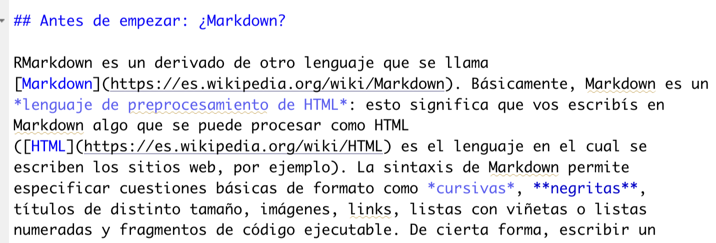
The title is marked with two ##s: a single symbol marks the largest title (called H1); The more symbols, the further down the title hierarchy. Then, the links have a double structure: the word we want to link in brackets and then the destination link in parentheses. Finally, asterisks are used to mark italics and bold. As you may have seen, Markdown is a very simple language and is designed to be easy to read.

R+Markdown

You don’t have to be a genius to understand, now, that RMarkdown is a version of Markdown that can be used with R. It is a type of file where we can write formatted text (that is, beautify it with italics, bold, titles, tables, bibliographic references, images; everything you would do in a Word document) and you can also add executable code and show the results. This document can also be processed as HTML (if you want to upload it to a blog), as PDF or as Word.

All of this facilitates reproducibility: the possibility of rerunning the same analysis and obtaining (or not) the same results. In general, there is a tendency to think of reproducibility as something important among researchers: Mary runs an investigation and finds X result; If someone else runs the same analysis with the same database, they should obtain the same result (if Mary was a sensible and transparent researcher). However, reproducibility is also important intra researchers: several times we find ourselves needing to rerun our same analyses, either because we find an error or because we modify the original amount of data. If the code in our analysis is clean and tidy, we will only need to replace the address of our database file and not touch anything else.

Before starting, we have to install two packages: knitr, which is used to build the files, and rmarkdown, which is the package that allows you to create the RMarkdown files. The code to install them is the following:

install.packages(c("knitr", "rmarkdown"))

Unlike other packages, these do not need to be loaded (with the library() function) every time we are going to use them, so once you install them you can forget about them.

Now, let’s get to work. RMarkdown is a type of file, therefore to generate it we go to File > New File > RMarkdown, or from the little white square with a + button green color. When you open it, the following will appear:

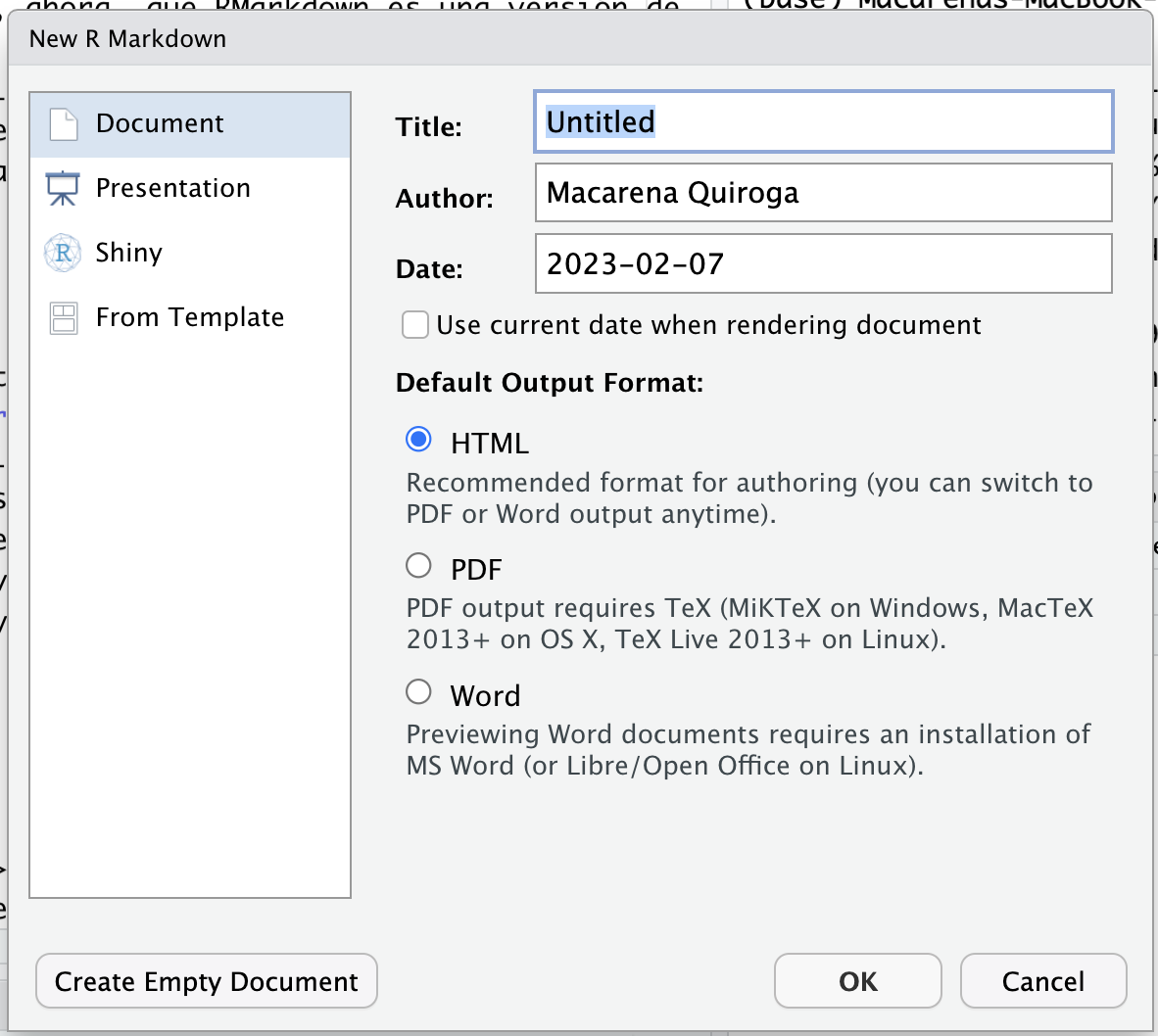
Everything that appears here you can change later, so my suggestion is to not overload your working memory and go aheand and select Ok. Anyway, you can now start to see what I mentioned before: from an RMarkdown you can export or convert your file to html, pdf or word. You can create documents, which is what we are going to do, but you can also create PowerPoint-type presentations, web applications with a package called Shiny, and you can also upload your own format templates. But for now, we are left with a basic document.

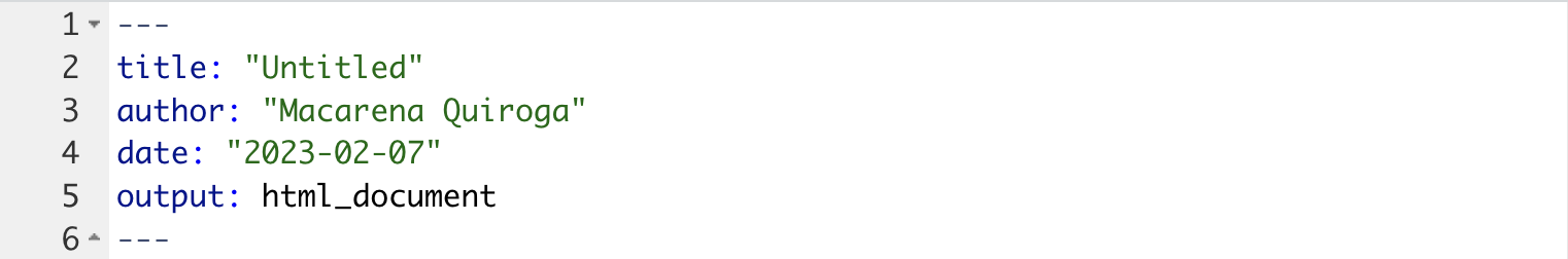
After pressing Ok, the RMarkdown document opens with a template, that is, a prefabricated model with some of Markdown’s own marks. There are three main types of important information:

1. The first segment of the first few lines, enclosed in dashes (---). It is called the YAML code block and it is where the general configuration of the document will be set. The information that we chose on the previous screen appears there by default, but we can also edit it by hand to add other things (like a subtitle, for example). The YAML format is very simple: words followed by a colon.

   

   YAML fragment

2. The second important segment is going to be the code blocks and you identify them because they begin with three inverted accents (or grave accents, for French-speaking people) ``` and because they appear in gray. The line between braces {} contains the information about how that block of code has to be executed. These blocks of code are called chunk and you can add more blocks with Code > Insert chunk or whatever keyboard shortcut shows you.

   

   R code chunk image.

3. Finally, everything that is outside of those blocks of code is the plain text, that is, the text that we can edit in Markdown to format it in the same way we work with a Word document.

   

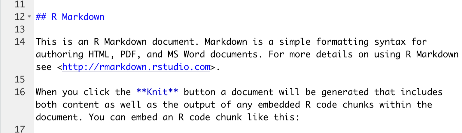   Image of the default text fragment.

And before seeing a little more how we can take advantage of this, I want you to see the magic of RMarkdown: click on the Knit button that is in the menu just above the document. It will ask you to name the file, then strange things will appear in the console and finally, in the viewer panel at the bottom right, you will have a preview of what that document would look like with the format applied.

And now?

Now, my suggestion is that you try modifying this template to see what happens. The model uses the cars dataframe, but you can add any code snippet you prefer. You can find more information on how to customize the text in this RStudio guide. In the next post we are going to see how we can customize an RMarkdown document, that is, how we can control what is shown and what is not, how to export it and other things.

As always, remember that you can subscribe to my blog so you don’t miss any updates , and if you have any questions, do not hesitate to contact me. And, if you like what I do, you can buy me a cafecito from Argentina or a kofi from other countries.